R for data science: Tidyverse

The tidyverse is one of the most popular ecosystems for data science in R. It includes many R packages commonly used in everyday data analysis. The core packages are as follows:

• ggplot2 for visualization

• dplyr for data manipulation

• tidyr to tidy your data

• readr to read data

• purrr for functional programming

• tibble for enhanced data frames

• stringr for string manipulation

• forcats for working with categorical data (factors)

Loading the tidyverse

The tidyverse is a collection of packages. In R, to load a library or package, you simply use the library() function. This is similar to using the import keyword in Python.

# install.packages("tidyverse")
library("tidyverse")

── Attaching core tidyverse packages ────────────────────────────────────────────────────────────────────────────────────────────────────────────────────────────────────────────────────────────────────────────────────────────────────────────────────────── tidyverse 2.0.0 ──
✔ dplyr     1.1.4     ✔ readr     2.1.5
✔ forcats   1.0.0     ✔ stringr   1.5.1
✔ ggplot2   3.5.1     ✔ tibble    3.2.1
✔ lubridate 1.9.3     ✔ tidyr     1.3.1
✔ purrr     1.0.2     

── Conflicts ──────────────────────────────────────────────────────────────────────────────────────────────────────────────────────────────────────────────────────────────────────────────────────────────────────────────────────────────────────────── tidyverse_conflicts() ──
✖ dplyr::filter() masks stats::filter()
✖ dplyr::lag()    masks stats::lag()
ℹ Use the conflicted package (<http://conflicted.r-lib.org/>) to force all conflicts to become errors

The pipe (%>%) operator

One of the most powerful tools introduced in the tidyverse is the pipe (%>%) operator, which enables chaining functions in a clear, readable way—especially useful for data manipulation tasks.

Here’s an example where we first apply a logical filter, then select specific columns, and finally sort the data:

# Example with the iris dataset
iris.df<-read.csv("https://raw.githubusercontent.com/mwaskom/seaborn-data/refs/heads/master/iris.csv")

iris.df.pipe <- # Save the resulting pipeline into this variable
    iris.df %>% # start with the original dataframe
        filter(species == "virginica") %>% # take observations corresponding to virginica
            select(petal_length, petal_width) %>%  # select petal_length and petal_width colums
                arrange(desc(petal_length)) # sort data in descending order based on petal_length

head(iris.df.pipe)

A data.frame: 6 × 2

	petal_length	petal_width
	<dbl>	<dbl>
1	6.9	2.3
2	6.7	2.2
3	6.7	2.0
4	6.6	2.1
5	6.4	2.0
6	6.3	1.8

Data cleaning

df.to.clean = data.frame(x = c(2, NA, 1, 1), 
                          y = c(NA, NA, 6, 6)
                         )
df.to.clean

A data.frame: 4 × 2

x	y
<dbl>	<dbl>
2	NA
NA	NA
1	6
1	6

drop_na: drop missing values

df.to.clean %>% drop_na()

A data.frame: 2 × 2

x	y
<dbl>	<dbl>
1	6
1	6

replace_na: replace missing values

df.to.clean %>%replace_na(list(x=0, y=0))

A data.frame: 4 × 2

x	y
<dbl>	<dbl>
2	0
0	0
1	6
1	6

distinc: drop duplicated data

df.to.clean %>% distinct()

A data.frame: 3 × 2

x	y
<dbl>	<dbl>
2	NA
NA	NA
1	6

Remember: we can concatenate them together.

df.to.clean %>% replace_na(list(x=0, y=0)) %>% distinct()

A data.frame: 3 × 2

x	y
<dbl>	<dbl>
2	0
0	0
1	6

Data manipulation

# let's load again our Iris dataframe
iris.df<-read.csv("https://raw.githubusercontent.com/mwaskom/seaborn-data/refs/heads/master/iris.csv")

dim(iris.df)

1. 150
2. 5

str(iris.df)

'data.frame':	150 obs. of  5 variables:
 $ sepal_length: num  5.1 4.9 4.7 4.6 5 5.4 4.6 5 4.4 4.9 ...
 $ sepal_width : num  3.5 3 3.2 3.1 3.6 3.9 3.4 3.4 2.9 3.1 ...
 $ petal_length: num  1.4 1.4 1.3 1.5 1.4 1.7 1.4 1.5 1.4 1.5 ...
 $ petal_width : num  0.2 0.2 0.2 0.2 0.2 0.4 0.3 0.2 0.2 0.1 ...
 $ species     : chr  "setosa" "setosa" "setosa" "setosa" ...

filter: Pick observations by their values

This function allows you to subset observations based on specific conditions.

iris.df.setosa<-iris.df %>% filter(species=="setosa")

head(iris.df.setosa)

A data.frame: 6 × 5

	sepal_length	sepal_width	petal_length	petal_width	species
	<dbl>	<dbl>	<dbl>	<dbl>	<chr>
1	5.1	3.5	1.4	0.2	setosa
2	4.9	3.0	1.4	0.2	setosa
3	4.7	3.2	1.3	0.2	setosa
4	4.6	3.1	1.5	0.2	setosa
5	5.0	3.6	1.4	0.2	setosa
6	5.4	3.9	1.7	0.4	setosa

# Here filtering based on two columns
iris.df.setosa.2<-iris.df %>% filter(species=="setosa", sepal_width>3)

head(iris.df.setosa.2)

A data.frame: 6 × 5

	sepal_length	sepal_width	petal_length	petal_width	species
	<dbl>	<dbl>	<dbl>	<dbl>	<chr>
1	5.1	3.5	1.4	0.2	setosa
2	4.7	3.2	1.3	0.2	setosa
3	4.6	3.1	1.5	0.2	setosa
4	5.0	3.6	1.4	0.2	setosa
5	5.4	3.9	1.7	0.4	setosa
6	4.6	3.4	1.4	0.3	setosa

# Here filtering with two logical conditions in the same column
iris.df.3<-iris.df %>% filter(sepal_width> 2 & sepal_width <= 3)

head(iris.df.3)

A data.frame: 6 × 5

	sepal_length	sepal_width	petal_length	petal_width	species
	<dbl>	<dbl>	<dbl>	<dbl>	<chr>
1	4.9	3.0	1.4	0.2	setosa
2	4.4	2.9	1.4	0.2	setosa
3	4.8	3.0	1.4	0.1	setosa
4	4.3	3.0	1.1	0.1	setosa
5	5.0	3.0	1.6	0.2	setosa
6	4.4	3.0	1.3	0.2	setosa

arrange: sort data by value

This function takes a dataframe, and a set of column names (or more complicated expressions) to order by (in ascending order by default). If more than one column name is provided, each additional column is used to break ties in the values of preceding columns.

# This sorts the data based on sepal length first and then sepal_width
iris.df.sorted<-iris.df %>% arrange(sepal_length, sepal_width)
head(iris.df.sorted)

A data.frame: 6 × 5

	sepal_length	sepal_width	petal_length	petal_width	species
	<dbl>	<dbl>	<dbl>	<dbl>	<chr>
1	4.3	3.0	1.1	0.1	setosa
2	4.4	2.9	1.4	0.2	setosa
3	4.4	3.0	1.3	0.2	setosa
4	4.4	3.2	1.3	0.2	setosa
5	4.5	2.3	1.3	0.3	setosa
6	4.6	3.1	1.5	0.2	setosa

If we want to reorder in descending order, we can use the function desc. This, in contrast to Python’s Pandas, can be specified to single columns:

# This sorts the data based on sepal length first, in descending order, and then sepal_width, in ascending order
iris.df.sorted<-iris.df %>% arrange(desc(sepal_length), sepal_width)
head(iris.df.sorted)

A data.frame: 6 × 5

	sepal_length	sepal_width	petal_length	petal_width	species
	<dbl>	<dbl>	<dbl>	<dbl>	<chr>
1	7.9	3.8	6.4	2.0	virginica
2	7.7	2.6	6.9	2.3	virginica
3	7.7	2.8	6.7	2.0	virginica
4	7.7	3.0	6.1	2.3	virginica
5	7.7	3.8	6.7	2.2	virginica
6	7.6	3.0	6.6	2.1	virginica

select: select columns

It allows you to pick a subset of variables.

# This selects columns by the given names of the columns. Here we just select sepal_length, sepal_width and species
iris.df.select<-iris.df %>% select(sepal_length, sepal_width, species)

head(iris.df.select)

A data.frame: 6 × 3

	sepal_length	sepal_width	species
	<dbl>	<dbl>	<chr>
1	5.1	3.5	setosa
2	4.9	3.0	setosa
3	4.7	3.2	setosa
4	4.6	3.1	setosa
5	5.0	3.6	setosa
6	5.4	3.9	setosa

If you want to select consecutive columns, we can use the : operator, as in vectors.

# This selects all columns between sepal_length and petal_width (inclusive)
iris.df.select.2<-iris.df %>% select(sepal_length:petal_width)

head(iris.df.select.2)

A data.frame: 6 × 4

	sepal_length	sepal_width	petal_length	petal_width
	<dbl>	<dbl>	<dbl>	<dbl>
1	5.1	3.5	1.4	0.2
2	4.9	3.0	1.4	0.2
3	4.7	3.2	1.3	0.2
4	4.6	3.1	1.5	0.2
5	5.0	3.6	1.4	0.2
6	5.4	3.9	1.7	0.4

And you can use a minus (-) operator before the name of the columns to filter them out.

# This selects all columns but sepal_length and sepal_width
iris.df.select.3<-iris.df %>% select(-sepal_length, -sepal_width)

head(iris.df.select.3)

A data.frame: 6 × 3

	petal_length	petal_width	species
	<dbl>	<dbl>	<chr>
1	1.4	0.2	setosa
2	1.4	0.2	setosa
3	1.3	0.2	setosa
4	1.5	0.2	setosa
5	1.4	0.2	setosa
6	1.7	0.4	setosa

And you can also remove consecutive columns by combining both operators:

iris.df.select.4<-iris.df %>% select(-(sepal_length:petal_width))

head(iris.df.select.4)

A data.frame: 6 × 1

	species
	<chr>
1	setosa
2	setosa
3	setosa
4	setosa
5	setosa
6	setosa

mutate: creating columns

This function allows you to add new columns to data frames. It would be mostly similar to assign in Python’s Pandas

# This creates a new column by multiplying summing sepal_length with sepal_width
iris.df.volume<-iris.df %>% mutate(sepal_volume=sepal_length*sepal_width)
head(iris.df.volume)

A data.frame: 6 × 6

	sepal_length	sepal_width	petal_length	petal_width	species	sepal_volume
	<dbl>	<dbl>	<dbl>	<dbl>	<chr>	<dbl>
1	5.1	3.5	1.4	0.2	setosa	17.85
2	4.9	3.0	1.4	0.2	setosa	14.70
3	4.7	3.2	1.3	0.2	setosa	15.04
4	4.6	3.1	1.5	0.2	setosa	14.26
5	5.0	3.6	1.4	0.2	setosa	18.00
6	5.4	3.9	1.7	0.4	setosa	21.06

We can always use a preceding created column to define a new column.

# This creates a new column by multiplying multiplying sepal_length with sepal_width, and a second column with the logarithm
iris.df.volume.2<- iris.df %>% mutate(sepal_volume=sepal_length*sepal_width, sepal_volume_log=log(sepal_volume))
head(iris.df.volume.2)

A data.frame: 6 × 7

	sepal_length	sepal_width	petal_length	petal_width	species	sepal_volume	sepal_volume_log
	<dbl>	<dbl>	<dbl>	<dbl>	<chr>	<dbl>	<dbl>
1	5.1	3.5	1.4	0.2	setosa	17.85	2.882004
2	4.9	3.0	1.4	0.2	setosa	14.70	2.687847
3	4.7	3.2	1.3	0.2	setosa	15.04	2.710713
4	4.6	3.1	1.5	0.2	setosa	14.26	2.657458
5	5.0	3.6	1.4	0.2	setosa	18.00	2.890372
6	5.4	3.9	1.7	0.4	setosa	21.06	3.047376

# Obviously, this is going to give an error because we are trying to use a sepal_volume before it was created
iris.df.volume.3<-iris.df %>% mutate(sepal_volume_log=log(sepal_volume), sepal_volume=sepal_length*sepal_width)
head(iris.df.volume.3)

Error in `mutate()`:
ℹ In argument: `sepal_volume_log = log(sepal_volume)`.
Caused by error:
! objeto 'sepal_volume' no encontrado
Traceback:

1. mutate(., sepal_volume_log = log(sepal_volume), sepal_volume = sepal_length * 
 .     sepal_width)
2. mutate.data.frame(., sepal_volume_log = log(sepal_volume), sepal_volume = sepal_length * 
 .     sepal_width)
3. mutate_cols(.data, dplyr_quosures(...), by)
4. withCallingHandlers(for (i in seq_along(dots)) {
 .     poke_error_context(dots, i, mask = mask)
 .     context_poke("column", old_current_column)
 .     new_columns <- mutate_col(dots[[i]], data, mask, new_columns)
 . }, error = dplyr_error_handler(dots = dots, mask = mask, bullets = mutate_bullets, 
 .     error_call = error_call, error_class = "dplyr:::mutate_error"), 
 .     warning = dplyr_warning_handler(state = warnings_state, mask = mask, 
 .         error_call = error_call))
5. mutate_col(dots[[i]], data, mask, new_columns)
6. mask$eval_all_mutate(quo)
7. eval()
8. .handleSimpleError(function (cnd) 
 . {
 .     local_error_context(dots, i = frame[[i_sym]], mask = mask)
 .     if (inherits(cnd, "dplyr:::internal_error")) {
 .         parent <- error_cnd(message = bullets(cnd))
 .     }
 .     else {
 .         parent <- cnd
 .     }
 .     message <- c(cnd_bullet_header(action), i = if (has_active_group_context(mask)) cnd_bullet_cur_group_label())
 .     abort(message, class = error_class, parent = parent, call = error_call)
 . }, "objeto 'sepal_volume' no encontrado", base::quote(NULL))
9. h(simpleError(msg, call))
10. abort(message, class = error_class, parent = parent, call = error_call)
11. signal_abort(cnd, .file)
12. signalCondition(cnd)

group_by and summarize: collapse down to a single summary

This would be similar to using groupby method in Pandas’ dataframes

# This first groups by species and then calculates the average sepal length within each category
iris.df %>% group_by(species) %>% summarize(mean_sepal_length = mean(sepal_length))

A tibble: 3 × 2

species	mean_sepal_length
<chr>	<dbl>
setosa	5.006
versicolor	5.936
virginica	6.588

# You can can have several aggregation methods too
iris.df %>% group_by(species) %>% summarize(mean_sepal_length = mean(sepal_length),
                                            median_sepal_length = median(sepal_length))

A tibble: 3 × 3

species	mean_sepal_length	median_sepal_length
<chr>	<dbl>	<dbl>
setosa	5.006	5.0
versicolor	5.936	5.9
virginica	6.588	6.5

If you want to apply the same aggregation method to several columns, you need to use the across function:

# This first groups by species and then calculates the average across all columns between sepal_length and petal_width
iris.df %>% group_by(species) %>% summarize(across(sepal_length:petal_width, mean)) 

A tibble: 3 × 5

species	sepal_length	sepal_width	petal_length	petal_width
<chr>	<dbl>	<dbl>	<dbl>	<dbl>
setosa	5.006	3.428	1.462	0.246
versicolor	5.936	2.770	4.260	1.326
virginica	6.588	2.974	5.552	2.026

pivot_longer: reshape data to long format

This would be similart to pd.melt in Python’s Pandas

iris.df.melt<-iris.df %>% pivot_longer(sepal_length:petal_width)

head(iris.df.melt)

A tibble: 6 × 3

species	name	value
<chr>	<chr>	<dbl>
setosa	sepal_length	5.1
setosa	sepal_width	3.5
setosa	petal_length	1.4
setosa	petal_width	0.2
setosa	sepal_length	4.9
setosa	sepal_width	3.0

Data visualization

I don’t want to finish this introduction to doing data science in R without briefly showing ggplot2.

ggplot2 is for data visualization, and personally, I think it is the best thing in R. It allows you to create magnificient and professional plots in an elegant and versatile way.

It is based on grammar of graphics, a coherent system for describing and building graphs.

To build a ggplot, you need to use the following basic template that can be used for different types of plots:

ggplot(data = <DATA>, mapping = aes(<MAPPINGS>)) +  <GEOM_FUNCTION>()

or

ggplot(data = <DATA>) +  <GEOM_FUNCTION>(mapping = aes(<MAPPINGS>))

In a nutshell:

• One begins a plot with the function ggplot, which creates a coordinate system where you can add layers to.

• The first argument of ggplot is the dataset to use in the graph.

• The graph can be then completed by adding one or more layers to ggplot using a geom function.

• Each geom function in ggplot2 takes a mapping argument. This defines how variables in your dataset are mapped to visual properties. The mapping argument is always paired with the function aes, and the x and y arguments of aes() specify which variables to map to the x- and y-axes.

• ggplot2 comes with many geom functions that each add a different type of layer to a plot

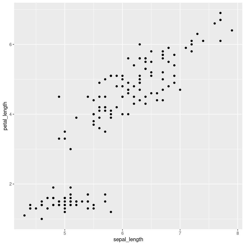
iris.df %>% ggplot(aes(x=sepal_length, y=petal_length)) + geom_point()

# or

iris.df %>% ggplot() + geom_point(aes(x=sepal_length, y=petal_length))

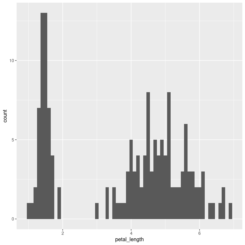
iris.df %>% ggplot(aes(x=petal_length)) + geom_histogram(binwidth = 0.1)

We can assign the plot to a variable and render it any time we like:

g <- iris.df %>% ggplot(aes(x=sepal_length, y=petal_length)) + geom_point()
g

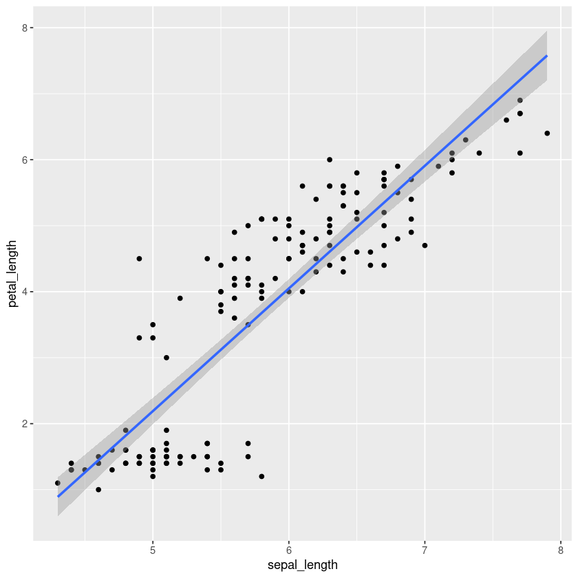
And we can keep adding layers to incorporate more graphics to the plot:

g + geom_smooth(method='lm')

`geom_smooth()` using formula = 'y ~ x'

The full list of available layers (geom_ functions) can be found at https://ggplot2.tidyverse.org/reference.

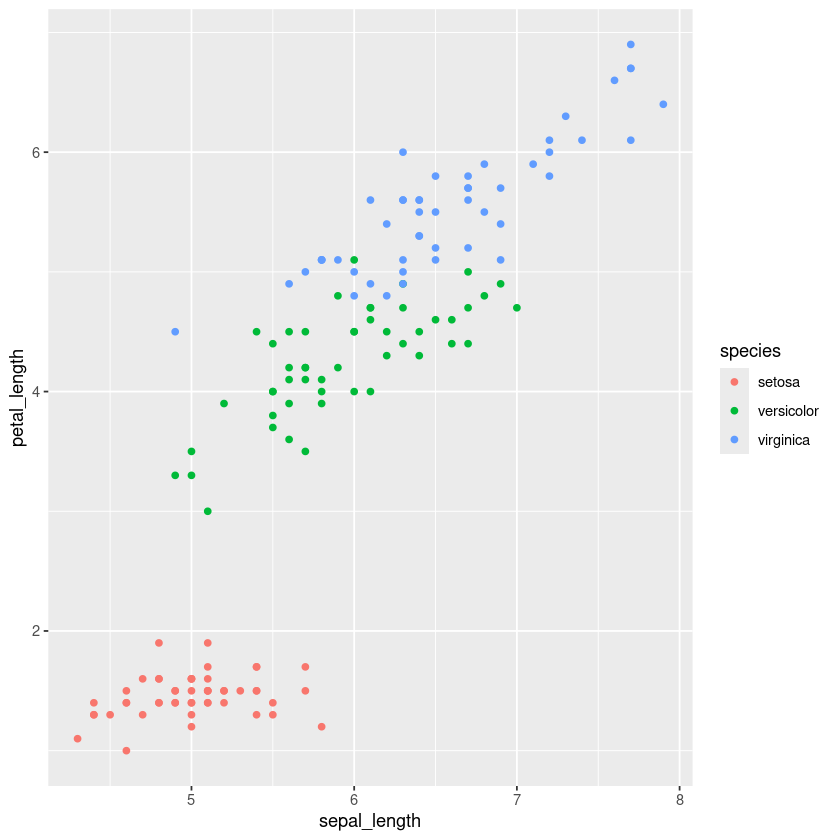
And as we mentioned, we can also control the aesthetics of the plot through the aes function. Examples of this include:

• Position (i.e., on the x and y axes)

• Color (“outside” color)

• Fill (“inside” color)

• Shape (of points)

• Alpha (Transparency)

• Line type

• Size

iris.df %>% ggplot(aes(x=sepal_length, y=petal_length, color=species)) + geom_point()

iris.df %>% ggplot(aes(x=sepal_length, y=petal_length, color=species, size=petal_width)) + geom_point()

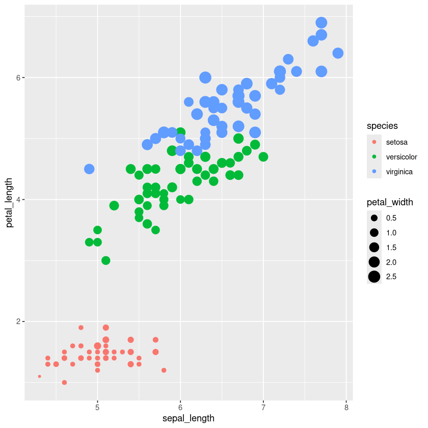
iris.df %>% ggplot(aes(x=petal_length, fill=species)) + geom_histogram(binwidth = 0.1)

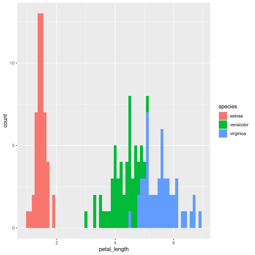
I recommend visiting the R graph gallery for a complete list of recipes on creating graphs using ggplot. You’ll have fun!

Practice exercises

Exercise 61

1- Import the data from “https://vincentarelbundock.github.io/Rdatasets/csv/psych/sat.act.csv”, which contains SAT and ACT scores for a sample of students. Save it to a variable named sat.dat.

2- Convert “education” and “gender” columns to factor type. (Hint: use as.factor function)

3- Using the pipe (%>%) operator, perform the following operations in sequence:

• Filter the data to include only observations where age is between 18 and 45 years.

• Create a new variable, SAT.avg, representing the average of SATQ and SATV.

• Select the columns gender, education, and SAT.avg.

• Group the dataframe by gender and education.

• Summarize the dataframe by computing the mean and standard deviation of SAT.avg. Here, since there are some missing information, you will need to remove these observations. You can actually do this when using the mean and sd functions. Look into their documentation to figure out how to do this.

Save the resulting dataframe in a variable named sat.dat.preprocessed and display it.

4- With the resulting dataframe, create a barplot using geom_bar:

• Set the x position to each level of education, and the height (y position) to the mean of SAT.avg.

• To display a separate bar for each gender, set fill = gender in the aesthetics, and use position = "dodge" to place the bars side by side rather than stacked.

Adjust the plot aesthetics to make it more visually appealing. You may find the following page useful for this: https://r-graph-gallery.com/4-barplot-with-error-bar.html

# Your answers from here