(This is simplified documentation from https://jupyter-notebook.readthedocs.io. You are more than welcome to visit the aforementioned page for more details)
Jupyter Notebooks#
Introduction#
The Jupyter Notebook is an interactive computing environment that enables users to author notebook documents that include:
Live code
Interactive widgets
Plots
Narrative text
Equations
Images
Video
Components#
The Jupyter Notebook combines three components:
The notebook web application: An interactive web application for writing and running code interactively and authoring notebook documents.
Kernels: Separate processes started by the notebook web application that runs users’ code in a given language and returns output back to the notebook web application. The kernel also handles things like computations for interactive widgets, tab completion and introspection.
Notebook documents: Self-contained documents that contain a representation of all content visible in the notebook web application, including inputs and outputs of the computations, narrative text, equations, images, and rich media representations of objects. Each notebook document has its own kernel.
Notebook documents#
When you run the notebook web application on your computer, notebook documents are just files on your local filesystem with a .ipynb extension. This allows you to use familiar workflows for organizing your notebooks into folders and sharing them with others.
Notebooks consist of a linear sequence of cells. There are three basic cell types:
Code cells: Input and output of live code that is run in the kernel
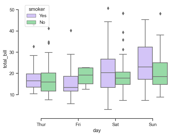
# This a code cell. Code rom https://seaborn.pydata.org/examples/grouped_boxplot.html
import seaborn as sns
sns.set_theme(style="ticks", palette="pastel")

# Load the example tips dataset
tips = sns.load_dataset("tips")

# Draw a nested boxplot to show bills by day and time
sns.boxplot(x="day", y="total_bill",
            hue="smoker", palette=["m", "g"],
            data=tips)
sns.despine(offset=10, trim=True)

Markdown cells: arrative text with embedded LaTeX equations
This is here is mardown. As such Markdown rules apply here!
Raw cells: Unformatted text that is included, without modification, when notebooks are converted to different formats using nbconvert
Notebook Basics#
Modal editor#
Jupyter Notebooks have a modal user interface, which means that the keyboard does different things depending on which mode the Notebook is in. There are two modes: edit mode and command mode.
Edit mode#
When in edit mode, cell’s borders become blue, background becomes white and a blinking cursor shows up. In this mode, you can type into the cell, like a normal text editor.
Note
In classic jupyter-notebooks this mode is indicated by a green cell borderand a prompt showing in the editor area.
Command mode#
When in command mode, blue borders become longer, the background grey, and the blinking cursor disappears. In this mode, you are able to edit the notebook as a whole, but not type into individual cells.
Note
In classic jupyter-notebooks this mode is indicated by a grey cell border with a blue left margin. When you are in command mode,
Most importantly, in command mode, the keyboard is mapped to a set of shortcuts that let you perform notebook and cell actions efficiently.
For example, if you are in command mode and you press c, you will copy the current cell - no modifier is needed.
Running Code (edit mode)#
Shift-Enteror pressing the button in the toolbar above runs a code cell.Alt-Enterruns the current cell and inserts a new one below.Ctrl-Enterrun the current cell and enters command mode.
Restarting the kernels#
The kernel maintains the state of a notebook’s computations. You can reset this state by restarting the kernel. This is done by clicking on the in the toolbar above.
Exercise 1
Create a cell below or above using either the keyworad with one of the shortcuts shown before, or using the menu with the mouse. Then, change to edit mode in the created cell and try introducing a number and running the cell using any of the above combinations. Do the same now, but changing the cell to markdown and typing some text in it.
More Resources#
Thorugh documentation: https://jupyter-notebook.readthedocs.io. I recommend checking the section dedicated to markdowns.
jupyter notebooks cheat sheet: https://www.edureka.co/blog/wp-content/uploads/2018/10/Jupyter_Notebook_CheatSheet_Edureka.pdf
